rm(list = ls())       ## create a clean environment

# create a dataframe called 'data'. The dataframe has 10 observations of 3 variables
data <- data.frame(
id = 1:10,
age = c(25, 31, 29, NA, 45, 38, NA, 52, 47, 33),
gender = c("M", "F", "F", "M", "F", NA, "M", "F", NA, "M")
)14 Data Pre-Processing
14.1 Learning Outcomes
By the end of this section, you should:
understand the importance of defining objectives for your analysis
understand how to deal with missing data in R
understand how to identify, and deal with, outliers in your dataset
14.2 Introduction
In my experience, much of your time as an analyst will be taken up with the data pre-processing stage (rather than actual analysis!). This stage involves cleaning, transforming, and organising the raw data into a suitable format for analysis. This often involves tasks such as handling missing values, normalisation, and encoding categorical variables.
This section works through the most common elements involved in data pre-processing, which you will be expected to apply during any analytic work you conduct.
14.3 Define Objectives for Your Analysis
At the outset, it is helpful to clearly outline the goals and objectives of your analysis, to guide the data pre-processing efforts. If you know what you want to analyse in the data, you can make quick decisions about (for example) whether to retain or discard certain variables within the dataset.
Some questions you will wish to think about (and perhaps discuss with others) are:
What’s the purpose of this analysis? It’s essential to know why the analysis is being conducted. For example, is it to inform a new playing strategy, to identify areas for individual improvement, or to solve a specific problem?
What are the key questions we want to answer? These questions will guide the entire analysis process. You should clearly understand what you’re looking to address (this helps you decide, for example, which variables to retain and which to remove from the dataset).
Who will use the findings from this analysis? The audience for your analysis can greatly influence how it’s conducted and how results will be presented. The needs of a management team might be different from those of a coaching team, for example. What do they need to see?
What decisions will be made based on this analysis? The end goal of most analysis is to inform decision-making. Understanding what those decisions might help you focus on the most relevant data.
What data do we need to conduct this analysis? The analyst needs to identify what data is required, where it can be obtained from, and if there are any potential challenges related to data collection or data quality.
Are there key metrics that we need to track? - These will help in quantifying the findings and tracking changes over time. It’s crucial to identify these early on, especially if you’re conducting the analysis as part of an ongoing training programme.
What are the potential biases or confounding factors? This was covered in the previous tutorial. Anticipating potential problems or limitations with the analysis can help avoid misguided conclusions.
What are the timelines for this analysis? Understanding the timeframes for delivery can help in planning and prioritising your work effectively. This is especially true in high-pressure environments such as professional sports clubs.
Are there any legal, ethical, or privacy considerations related to the analysis? Data analysis often involves sensitive information. It’s crucial to understand any relevant legal or ethical boundaries.
How will success be measured? Knowing what a successful outcome looks like can help guide the analysis and provide a clear target to aim for. This could be a specific improvement in a key metric, a problem solved, or a decision made. We’ll discuss this in greater detail in the following tutorial on Prescriptive Analytics.
14.4 Dealing with Missing Data
This is a critical phase of preparation- decisions made here can have a significant impact on subsequent analysis.
Failing to deal with missing data can basically invalidate your entire analysis.
Introduction
It’s common in sport data to have missing values. For example, an athlete may have missed a particular testing session, a team member may not have returned a value for one of the variables being collected, or the wearable device might have failed to collect measurements at particular points.
As an analyst, it’s important to identify any missing data and decide how to deal with it. This is particularly important when you have imported the dataset from another format, which may treat missing data differently to how it should be indicated in R.1
Initial Phase
At this stage, we’re looking to see how much data is missing in our dataset, and where these gaps exist. Later (Section 14.4.4), we’ll explore how to deal with instances of missing data.
Usefully, in R, you can identify missing data using the is.na() function, which returns a logical vector of the same dimensions as your input data with TRUE values for missing data (represented as NA) and FALSE values for non-missing data.
Important
Note that R will usually enter ‘NA’ into the field of any missing data in an imported dataset. It’s important to check that this has happened when you first import the dataset (e.g., using the ‘head’ command or opening the dataset in a tab).
Here’s an example of identifying missing data in a dataset:
First, I’ll create a synthetic dataset with three variables that have some missing values (‘NA’).2
In this dataset, there is a variable called [id] which is a vector from 1:10 (i.e., 1,2,3,..10).
There is a variable called [age] which you can see has two missing values (NA). Remember: R will assign the value NA to any element (cell) that has missing data.
There is a variable called [gender] which also has two missing values.
Identifying Missing Data
If we have a very small dataset, it’s easy to visually inspect the dataset and spot missing values. However, with large datasets, this becomes incredibly time-consuming and, even if we spot them, we still have to deal with them!
There are therefore several different techniques we need to learn that can be used to identify missing data in a dataset:
Technique 1 - using the is.na function
missing_data <- is.na(data)  # create a logical vector with TRUE or FALSE for each observation
print(missing_data) # show results in the console
id age gender
[1,] FALSE FALSE FALSE
[2,] FALSE FALSE FALSE
[3,] FALSE FALSE FALSE
[4,] FALSE TRUE FALSE
[5,] FALSE FALSE FALSE
[6,] FALSE FALSE TRUE
[7,] FALSE TRUE FALSE
[8,] FALSE FALSE FALSE
[9,] FALSE FALSE TRUE
[10,] FALSE FALSE FALSETechnique 2 - using the complete.cases function
complete.cases(data) [1] TRUE TRUE TRUE FALSE TRUE FALSE FALSE TRUE FALSE TRUE# shows whether each case is completed or not - printed to the console automaticallyTechnique 3 - also using the complete.cases function
data[!complete.cases(data),] id age gender
4 4 NA M
6 6 38 <NA>
7 7 NA M
9 9 47 <NA># This command shows the rows that have an NA in them. Note that we use the ! command in R to ask it find things that do NOT match our criteria, so in this case it has identified rows that are NOT complete cases.In the above example, the first option (using missing_data) created a logical matrix called [missing_data] which has the same dimensions as data, with TRUE values for missing data (i.e. is missing) and FALSE values for non-missing data (i.e. is not missing).
From this new matrix, we can calculate the total number of missing values in the dataset:
total_missing_values <- sum(missing_data) # the sum command is used to calculate a total and put it into a new object
print(total_missing_values)
[1] 4We can calculate the number of missing values in each variable (column):
missing_values_per_variable <- colSums(missing_data)
print(missing_values_per_variable)
id age gender
0 2 2 We can also calculate the proportion of missing values in each variable. If a large proportion of values are missing from a particular variable, this may raise questions about its retention.
proportion_missing_values <- colMeans(missing_data)
print(proportion_missing_values)
id age gender
0.0 0.2 0.2 In this case, we can see that 20% of our cases (rows) have missing data in the [age] variable, and 20% have missing data in the [gender] variable.
These steps help us identify missing data in the dataset and to understand the extent of ‘missingness’ in the data. Depending on the amount and pattern of missing data, we can decide on the most appropriate way to handle the missing data.
Handle any missing values
So we have a problem in our dataset. Some elements contain missing values.
If we’ve identified that there is missing data in our dataset, we now need to decide on the appropriate strategy to address missing data.
There are two main approaches to doing so:
One, called ‘imputation’, means that we create values and insert them in the missing spaces. We impute a value to replace the missing value.
The other approach is to remove records/observations where a missing value is present. In other words, if there’s a missing value, we ignore that observation (or delete it).
Tip
This is a complex issue and you should follow-up on this in your own time. For example, the ‘factual analysis’ method described below is useful where you know what the missing value should be.
Here are some of the techniques you may wish to follow-up. We’ll cover these in greater detail in the module B1705, during Semester 2.
Listwise Deletion: This involves removing the entire row of data if any single value is missing. It’s the simplest approach but can result in significant data loss.
Pairwise Deletion: This involves analysing all cases where the variables of interest are present and ignoring missing values. This is more efficient than listwise deletion because we don’t get rid of any observations, but can lead to biased results if the missing data isn’t completely random.
Mean/Median/Mode Imputation: Replacing missing values with the mean (for numerical data), median (for ordinal data), or mode (for categorical data) of the available values. This is easy to implement but can distort the distribution of data.
Predictive Imputation: Using statistical models like linear regression or machine learning techniques to predict and fill missing values based on other available data. This can be more accurate but requires robust models and significant computation.
Last Observation Carried Forward/Next Observation Carried Backward (LOCF/ NOCB): This is commonly used in time-series data where the missing value is filled with the last observed value or the next observed value. So for example, if we are missing data from an athlete for week 4, but we have that data for week 3, we could enter the same data into week 4.
Multiple Imputation: Generating multiple possible values for the missing data, creating multiple “complete” datasets, analysing each dataset separately, and then pooling the results. This technique is statistically sound and reduces bias but is complex to implement.
Interpolation: This method is mainly used in time series data, where missing values are filled based on the values in adjacent periods. In other words, we create a value for the ‘missing’ value that leads us from the previous value to the next value (e.g. 50 -75 - 100, assuming the middle observation was missing).
Hot Deck Imputation: Randomly choosing a value from a similar observation to replace the missing data. It’s more sophisticated than mean imputation but can still introduce bias.
Note
For the remainder of this module, we will assume that the best approach is ‘listwise deletion’. This means that we delete any observations (rows) where there is a missing value in any of the cells. The problem with this approach is that, in smaller datasets, it may mean you get rid of lots of observations, thus reducing your dataset to a dangerously small level.
The simplest way to carry out listwise deletion is with the na.omit command, as shown in the following code. You’ll see that it simply removes all the rows where there were missing values in **any* of the elements.
data01 <- na.omit(data)  # creates new datafame called data01 with only complete observations
print(data01)  # the resulting dataset is printed to the console.
id age gender
1 1 25 M
2 2 31 F
3 3 29 F
5 5 45 F
8 8 52 F
10 10 33 M
Note
In the previous example, I created a new dataframe called ‘data01’ which had the missing observations removed. This is better than simply overwriting the existing dataframe (‘data’) as I might wish to return to that original dataframe later in the analysis.
Conclusion
In this section, we’ve discussed two main things: how to identify if there is missing data present in our dataset, and how to remove any rows that contain missing data.
14.5 Outlier Detection
‘Outliers’ are data points that significantly differ from the rest of the data. They are often caused by errors in data collection or data entry (the analyst enters 99 instead of 9), or they may represent genuine variations within the data (a player has an exceptional performance in a single game).
Detecting outliers is essential because they can have a strong influence on the results of data analysis and lead to misleading conclusions. However, it may not always be clear whether a value is a mistake, or if it represents a genuine observation.
There are two types of approach to inspecting for outliers - visual and statistical - that we can use to detect outliers in a dataset.
Visual methods
By plotting variables in our data, we can easily detect the presence of outliers. The most common methods used for this are box plots, scatter plots, and histograms.
In the following examples I’ve used a version of the dataset we used earlier in the module. In this version, I have introduced some outliers.
rm(list = ls())       ## create a clean environment
url <- "https://www.dropbox.com/scl/fi/jb9b9uhx728e4h6g46r1n/t10_data_b1700_02.csv?rlkey=3sjwjwd6y59uj5lq588eufvpm&dl=1"
df <- read.csv(url)
rm(url)
Box plots
Box plots are useful because they give us a visual indication of a variable’s characteristics (25th percentile, 50th percentile, 75th percentile, minimum, maximum and maximum values). They also show any observations that lie ‘outside’ of that range.
Note the use of the
df$Plcommand - this tells R that we want to use the variable Pl in the df dataset. It’s important to remember what this means.
# create boxplot for the variable Pl, part of the df dataset

boxplot(df$Pl, main = "Box Plot - Outlier Detection")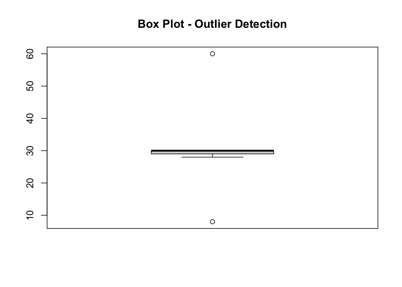
The resulting figure shows that there are two outliers within the variable ‘Pl’. One seems a lot greater than the rest of the observations, and one seems a lot less.
Scatter plots
In general a scatter plot is useful if you expect a general trend between two variables.
For example, in our dataset for the EPL, we would expect a team’s position in the league and its total number of lost games to be negatively associated (higher position = fewer losses). If we find this isn’t the case for certain teams, it suggests an outlier in the data.
# create scatter plot

plot(df$Pos, df$L, main = "Number of lost games by league position",
xlab = "League position", ylab = "Number of losses",
pch = 19, frame = FALSE)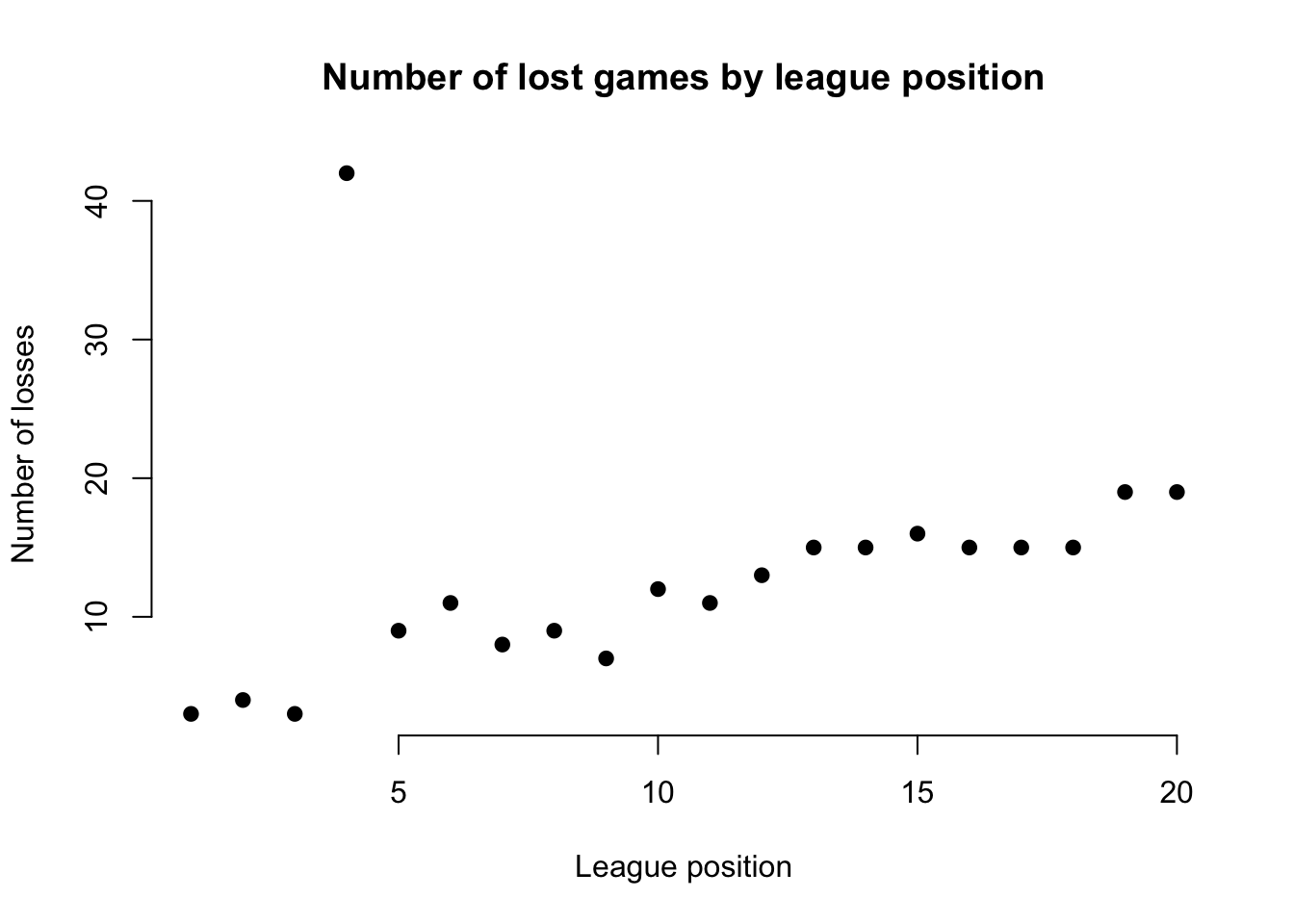
The resulting figure suggests an outlier in the data for the team at league position 4, whose number of lost games is far too high to be ‘reasonable’. It doesn’t mean it is definitely an outlier, but it may suggest further inspection.
Histograms
The previous techniques work if we’re dealing with scale/ratio types of data. However, we also want to visually explore outliers in categorical or ordinal data.
Therefore, if we can make a reasonable assumption about the frequency of values in a variable, we can use a histogram to explore outliers in that variable.
For example, in the current dataset, we would assume that every team will have drawn a roughly similar number games. By creating a histogram, we can identify potential outliers.
# create histogram

hist(df$D, col = "steelblue")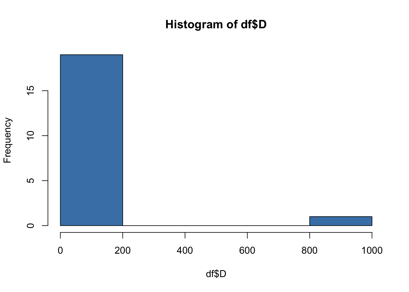
Clearly, there is a outlier in the ‘D’ variable! The x-axis shows that frequency of draws for most of our observations is in the range 0-200, while the frequency of draws for at least one of our observations is in the range 800-1000. We know that this cannot be correct!
Using the summary command
We’ve covered three visual approaches to outlier detection that involved plotting graphs.
We can also visually inspect the descriptive statistics of our variables. Note that this is a far quicker way to inspect the whole dataset, rather than plotting individual graphs for each variable.
By running the summary command, we can quickly see descriptive statistics for each variable.
This gives us another way to quickly identify potential outliers, as can be seen for the ‘D’ variable in the following example, which has a maximum of 999, or the ‘Pl’ variable which indicates the number of games played, and you know that teams don’t play 60 games in a season.
summary(df) Pos Team Pl W
Min. : 1.00 Length:26 Min. : 8.00 Min. : 6.00
1st Qu.: 5.75 Class :character 1st Qu.:29.00 1st Qu.: 7.75
Median :10.50 Mode :character Median :30.00 Median :10.00
Mean :10.50 Mean :30.05 Mean :11.30
3rd Qu.:15.25 3rd Qu.:30.00 3rd Qu.:14.25
Max. :20.00 Max. :60.00 Max. :23.00
NA's :6 NA's :6 NA's :6
D L F A
Min. : 4.0 Min. : 3.00 Min. :23.00 Min. :21.00
1st Qu.: 5.0 1st Qu.: 8.75 1st Qu.:28.25 1st Qu.:35.50
Median : 6.5 Median :12.50 Median :40.50 Median :40.00
Mean : 56.3 Mean :13.05 Mean :42.06 Mean :39.83
3rd Qu.: 9.0 3rd Qu.:15.00 3rd Qu.:49.50 3rd Qu.:42.75
Max. :999.0 Max. :42.00 Max. :75.00 Max. :54.00
NA's :6 NA's :6 NA's :8 NA's :8
GD Pts
Min. :-30.00 Min. :23.00
1st Qu.:-15.75 1st Qu.:29.75
Median : -1.50 Median :39.00
Mean : 0.00 Mean :40.90
3rd Qu.: 13.50 3rd Qu.:48.50
Max. : 48.00 Max. :73.00
NA's :6 NA's :6 Statistical methods
The previous methods depend on visual inspection, and are effective where there are very obvious outliers that are easily spotted.
A more robust approach to outlier detection is to use statistical methods, two of which (z-score and IQR) are outlined below. There are other, more complex, approaches you can follow-up if you wish.
We’ll cover this in greater detail in B1705, but basically we are attempting to evaluate whether a given value is within an acceptable range. If it is not, we are making a determination that this value is probably an outlier.
There are two techniques we commonly use for this: z-scores, and the IQR.
z-score
Z-scores represent how many standard deviations a data point is from the mean.
A common practice is to treat data points with z-scores above a certain absolute threshold (e.g., 2 or 3) as outliers.
library(zoo) # load the zoo package
Attaching package: 'zoo'The following objects are masked from 'package:base':
as.Date, as.Date.numeric # first we create some data - a set of values that all seem quite 'reasonable'.
data <- c(50, 51, 52, 55, 56, 57, 80, 81, 82)
# then, we calculate the z-scores for each value
z_scores <- scale(data) # we scale the data
threshold = 2 # we set an acceptable threshold for variation
outliers_z <- data[abs(z_scores) > threshold] # we identify values that sit outside that threshold
print(outliers_z) # there are no outliers in the datanumeric(0)data <- c(50, 51, 52, 55, 56, 57, 80, 81, 182) # Now, we introduce an outlier - 182 - to the vector
z_scores <- scale(data)
threshold = 2
outliers_z <- data[abs(z_scores) > threshold]
print(outliers_z) # note that the outlier has been identified successfully[1] 182Interquartile Range (IQR)
The interquartile range tells us the spread of the middle half of our data distribution.
Quartiles segment any vector that can be ordered from low to high into four equal parts. The interquartile range (IQR) contains the second and third quartiles, or the middle half of your data set.
In this method, we define outliers as values below (Q1 - 1.5 x IQR) or above (Q3 + 1.5 x IQR).
# Calculate IQR of our vector

Q1 <- quantile(data, 0.25)
Q3 <- quantile(data, 0.75)
IQR <- Q3 - Q1

# Define threshold (e.g., 1.5 times IQR)
lower_bound <- Q1 - 1.5 * IQR
upper_bound <- Q3 + 1.5 * IQR

# Identify outliers
outliers <- data[data < lower_bound | data > upper_bound]

# Print outliers
print(outliers)  # the outlier of 182 has been successfully identified
[1] 18214.6 Outlier Treatment
Similar to dealing with missing data, simply knowing that outliers exist doesn’t really help us! We need to find a way to tackle any outliers in our dataset.
Remove outliers
The easiest approach, as was the case with missing data, is to simply remove them.
Previously, we learned some approaches to visually identifying outliers. If we’ve done this, we can use the following process to ‘clean’ our data, because we know what the outlier value is.
data <- c(50, 51, 52, 55, 56, 57, 80, 81, 182)
data_clean <- data[data != 182] # here I've used the ! command to say [data_clean] is [data] that is NOT 182
If we’ve visually identified an outlier and know its index (position), for example through a scatter plot, we can remove it using its index:
data <- c(50, 51, 52, 55, 56, 57, 80, 81, 182)
data_clean <- data[-9] # this creates a new dataframe without the 9th element
print(data_clean)
[1] 50 51 52 55 56 57 80 81If using z-scores, we can use the following process, which assumes a threshold of 2 (we can adjust this based on our needs). Now, we can remove data points with z-scores greater than 2 in absolute value.
Notice that this is more efficient, because we don’t need to tell R what the value/s of the outliers are.
data <- c(50, 51, 52, 55, 56, 57, 80, 81, 182) # Example data with the 182 outlier
z_scores <- scale(data) # calculate z-scores
threshold = 2  # set threshold
data_cleaned <- data[abs(z_scores) <= threshold] # create a 'clean' set of data
print(data_cleaned) # the outlier has been removed
[1] 50 51 52 55 56 57 80 81Finally, we may want to remove all observations in a dataframe that contain an outlier in **any* column. This is helpful if we wish to retain the integrity of our dataframe rather than dividing it up into separate vectors.
# First, I create a sample dataframe with numeric data
df <- data.frame(
  Age = c(25, 30, 35, 40, 45, 50, 55, 60, 65, 999),
  Income = c(1800, 45000, 50000, 55000, 60000, 65000, 70000, 75000, 80000, 85000)
)

# This function can be used to remove outliers using z-scores
remove_outliers <- function(df, columns, z_threshold = 2) {
  df_cleaned <- df
  for (col in columns) {
    z_scores <- scale(df[[col]])
    outliers <- abs(z_scores) > z_threshold
    df_cleaned <- df_cleaned[!outliers, ]
  }
  return(df_cleaned)
}

# Now, specify the columns for which we want to remove outliers
columns_to_check <- c("Age", "Income")

# Remove outliers from the specified columns and create a 'cleaned'
# dataframe
df_cleaned <- remove_outliers(df, columns_to_check)

# Remove any observations (rows) with missing values
df_cleaned <- na.omit(df_cleaned)

# Print the cleaned dataframe
print(df_cleaned)
Age Income
2 30 45000
3 35 50000
4 40 55000
5 45 60000
6 50 65000
7 55 70000
8 60 75000
9 65 80000